The Secret of Statistical Transformations: Why Do We Need Monotonic Functions and Partitions?
When dealing with probability and statistics, we often need to transform a random variable $X$ into a new format, $Y = g(X)$. If our transformation is a simple linear equation like $Y = 2X + 3$, life is easy.
But what if our function is non-linear and wavy, like $Y = X^2$ or $Y = \sin(X)$? That is where we run into deep trouble. In this post, based on my personal study notes, we will explore why we desperately need the concept of “Monotonicity” and why we must divide the $X$-axis into “Partitions” to survive these transformations.
The Problem: Why Can’t We Just Take the Inverse?
The fundamental rule for transforming Probability Density Functions (PDFs) involves finding the inverse of our function, $x = g^{-1}(y)$, and plugging it into the formula.
However, there is a catch: You can only find a unique inverse for a function if it is strictly monotonic (meaning it only increases or only decreases).
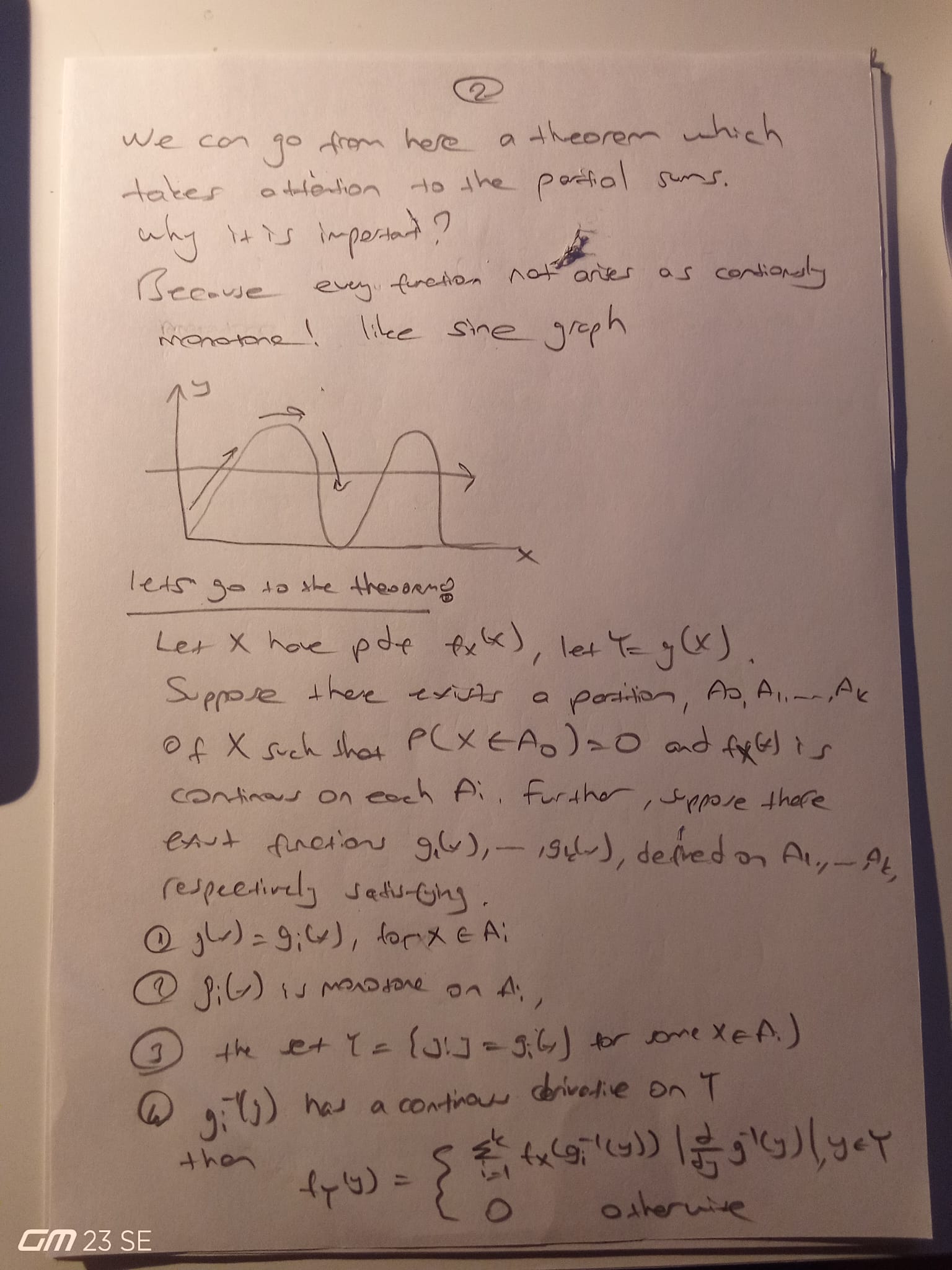 Figure 1: If a function is not continuously monotonic (like a sine wave), a horizontal line will intersect the curve at multiple points.
As you can see in my sketch above, if we draw a horizontal line across a non-monotonic graph, it intersects the curve at multiple points. This means a single $y$ value corresponds to multiple $x$ values. Which inverse function are we supposed to use?
The Solution: The “Divide and Conquer” Theorem
If the entire function is not monotonic, we simply divide the function into intervals where it IS monotonic. This is exactly what the daunting statistical theorem for transformations (often involving sums and partitions) tells us to do.
We partition the sample space into sets $A_1, A_2, \dots, A_k$ such that the function is strictly increasing or decreasing within each set. Then, we calculate the probabilities for each piece separately and sum them up.
Seeing the Math: The Square Transformation ($Y = X^2$)
Let’s prove the logic behind this partitioning using one of the most famous transformations: squaring a random variable.
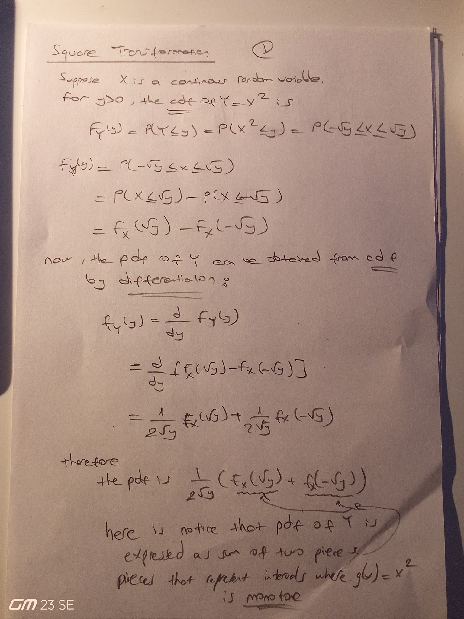 Figure 2: Deriving the PDF of $Y=X^2$ using the Cumulative Distribution Function (CDF) method.
As shown in my notes, we can start from the Cumulative Distribution Function (CDF):
- Our goal is to find $P(Y \le y)$. Substituting $X^2$ for $Y$, we get $P(X^2 \le y)$.
- Solving this inequality gives us boundaries for $X$: between $-\sqrt{y}$ and $+\sqrt{y}$. Notice how two roots (two separate partitions) naturally emerge!
- We write the CDF as: \(F_Y(y) = F_X(\sqrt{y}) - F_X(-\sqrt{y})\)
- To find the PDF, we differentiate the CDF with respect to $y$. Applying the chain rule, we get: \(f_Y(y) = \frac{1}{2\sqrt{y}} f_X(\sqrt{y}) + \frac{1}{2\sqrt{y}} f_X(-\sqrt{y})\)
The Key Takeaway: Notice how the final PDF of $Y$ is expressed as the sum of two pieces. These pieces directly represent the two intervals where $g(x) = X^2$ is monotonic (the left side of the parabola and the right side)! The $\frac{1}{2\sqrt{y}}$ terms are simply the absolute derivatives, acting as scaling factors for how much the space is stretched at those points.
The Holy Grail: From Standard Normal to Chi-Squared
Where is this heavily used in the real world? It is the exact mathematical mechanism used to transition from the Standard Normal Distribution ($Z$) to the Chi-Squared ($\chi^2$) distribution—a cornerstone of variance analysis and machine learning.
If you take a standard normal random variable and square it ($Y = X^2$), the resulting distribution is a Chi-Squared distribution with 1 degree of freedom. Let’s prove this using the partition theorem we just discussed.
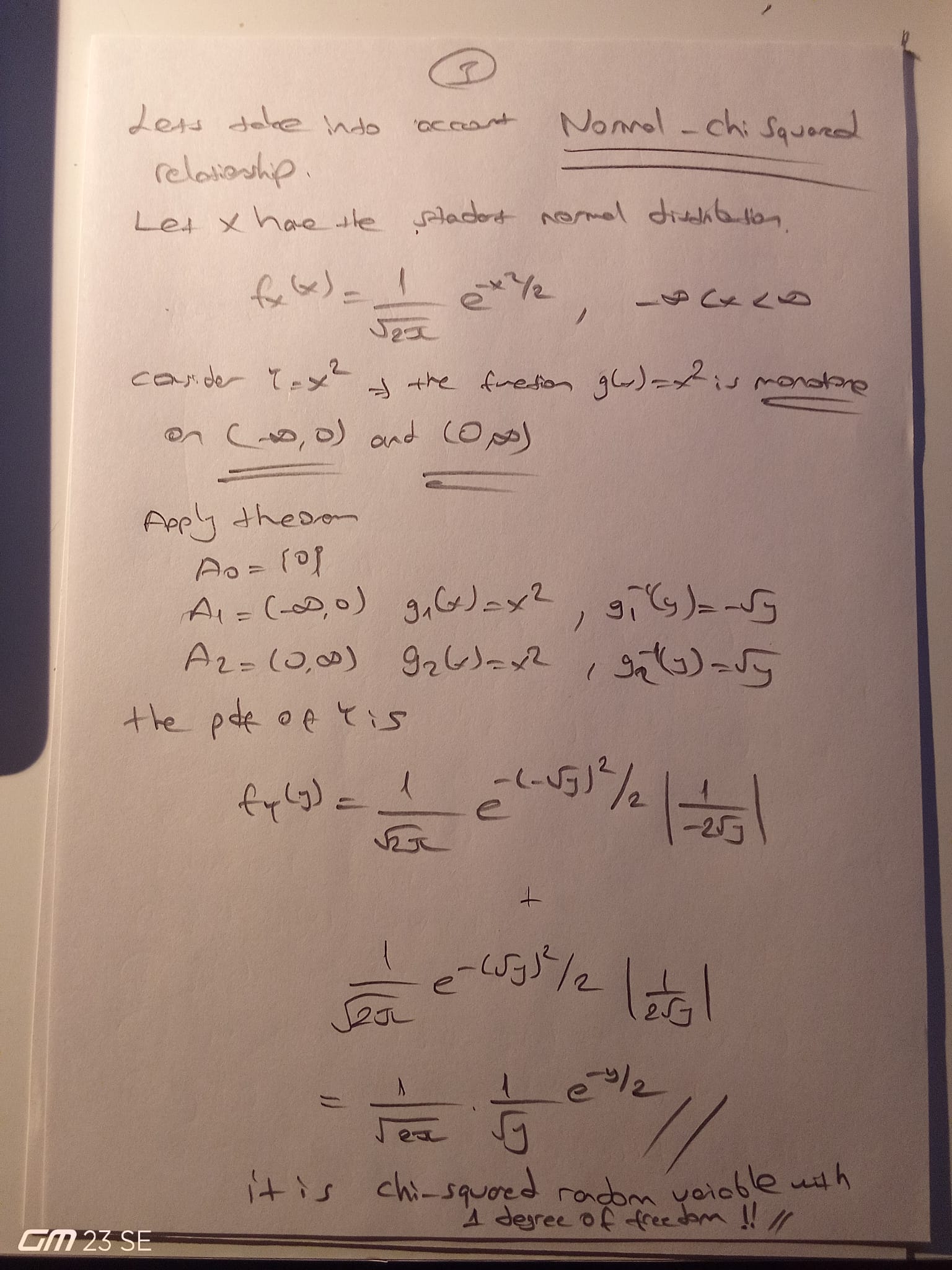 Figure 3: Applying the partition theorem to the Standard Normal PDF.
The steps are clear:
- The standard normal distribution is a bell curve. Due to the $X^2$ transformation, we divide it into two monotonic partitions: $A_1 = (-\infty, 0)$ and $A_2 = (0, \infty)$.
- The inverse functions for these partitions are $g_1^{-1}(y) = -\sqrt{y}$ and $g_2^{-1}(y) = \sqrt{y}$, respectively.
- The PDF of the standard normal distribution is: \(f_X(x) = \frac{1}{\sqrt{2\pi}} e^{-x^2/2}\)
-
We apply the theorem by plugging our inverse functions into the Normal PDF and multiplying by the absolute value of their derivatives $\left\lvert \frac{d}{dy} g^{-1}(y) \right\rvert$:
\[f_Y(y) = \frac{1}{\sqrt{2\pi}} e^{-(-\sqrt{y})^2/2} \left\lvert -\frac{1}{2\sqrt{y}} \right\rvert + \frac{1}{\sqrt{2\pi}} e^{-(\sqrt{y})^2/2} \left\lvert \frac{1}{2\sqrt{y}} \right\rvert\] -
Because the normal distribution is perfectly symmetrical, these two ugly pieces are identical. When we add them together, the 2’s in the denominator cancel out, leaving us with a beautiful, simplified formula:
\[f_Y(y) = \frac{1}{\sqrt{2\pi}\sqrt{y}} e^{-y/2} \quad \text{for } y > 0\]
And there it is! That simplified equation is the exact Probability Density Function of a Chi-squared random variable with 1 degree of freedom.
Conclusion
The intimidating formulas in statistics textbooks filled with summation symbols ($\Sigma$) and absolute derivatives are not arbitrary mathematical torture. When a function wavers up and down, those symbols are simply the mathematical instructions to: “Slice the graph into predictable pieces, calculate the stretched probability for each piece, and add them all together.”
Reference : Casella & Berger - Statistical Inference Book